PACMAN Control File (.pcf)
To run the different stages of PACMAN,
the pipeline requires a so-called PACMAN control file (.pcf)
where stage-specific parameters are defined (e.g. aperture size, path to the data, etc.).
In the following, we look at the contents of the pcf and include an example entry.
# This is the pcf file
# NOTE: DO NOT USE SPACES IN LISTS!

# 00
rundir                       /Users/sebastianzieba/Desktop/Projects/Observations/Hubble/GJ1214_13021_2026 # location of run dir
datadir                      /Users/sebastianzieba/Desktop/Data/GJ1214_Hubble13021        # location of data dir
suffix                       ima                                                # data suffix (only ima supported right now)
which_visits                 [5,6]                                          # which visits to use; Options: list (e.g., [0,1,3]) or everything

save_obs_times_plot          True
show_obs_times_plot          False


## 02 barycorr
save_barycorr_plot           True                                               # save a plot with locations of HST?
show_barycorr_plot           False


## 03
Teff                         3250                                               # effective temperature of the star
logg                         5.026                                              # surface gravity of the star
MH                           0.29                                               # metallicity of the star
sm                           k93models                                          # stellar model. Options: blackbody, k93models, ck04models or phoenix

smooth                       True                                               # smooth stellar spectrum using a gaussian kernel
smooth_sigma                 441

save_smooth_plot             True
show_smooth_plot             False

save_refspec_plot            True                                               # save a plot showing the stellar model, bandpass and the product of them?
show_refspec_plot            False

## 10
di_rmin                      120                                                # coordinates (row min max and column min max) where the star in the direct image is
di_rmax                      160
di_cmin                      5
di_cmax                      50

save_image_plot              True                                               # save plot with direct image and best fit?
show_image_plot              False

di_multi                     median


## 20
s20_testing                  False
n_testing                    4

rmin                         5
rmax                         261

window                       12

opt_extract                  True
sig_cut                      15                                                 # optimal extraction, for cosmic rays etc
nsmooth                      9                                                  # optimal extraction, created smoothed spatial profile, medial smoothing filter

correct_wave_shift           True
correct_wave_shift_refspec   True

background_thld              1000                                               # background threshold in counts

background_box               False
bg_rmin                      100
bg_rmax                      400
bg_cmin                      40
bg_cmax                      100

calculate_rowshift           True                                             # calculates spatial shift of spectrum on detector with respect to first exposure

save_rowshift_plot           True                                             # save plot of rowshift fit
show_rowshift_plot           False

save_rowshift_stretch_plot   True                                             # save plot of stretch fit and plot of profile stretch to rowshift
show_rowshift_stretch_plot   False

save_optextr_plot            False

save_sp2d_plot               False                                              # save plot of 2d spectrum
show_sp2d_plot               False

save_trace_plot              False                                              # save plot of trace
show_trace_plot              False

save_bkg_hist_plot           False                                              # save histogram of fluxes
show_bkg_hist_plot           False

save_utr_plot                False                                              # save plot of individual up-the-ramps
show_utr_plot                False

save_sp1d_plot               False                                              # save plot of 1d spectrum
show_sp1d_plot               False

save_bkg_evo_plot            True                                               # save plot of the background flux over time
show_bkg_evo_plot            False

save_sp1d_diff_plot          False                                              # save difference plot of consecutive 1d spectra
show_sp1d_diff_plot          False

save_utr_aper_evo_plot       True                                               # save plot of aperture size over time
show_utr_aper_evo_plot       False

save_refspec_fit_plot        True                                              # save plot of fit of the 1d spectrum to the refspec
show_refspec_fit_plot        False

save_drift_plot              True                                               # save plot of 1d spectrum drift over time
show_drift_plot              False


##21
wvl_min                      1.135
wvl_max                      1.642
wvl_bins                     11

use_wvl_list                 False
wvl_edge_list                [11400,12200,12600,13000,14600,15000,15400,15800,16200]


##30
#s30_myfuncs                  ['constant','upstream_downstream','model_ramp','polynomial1','transit']
s30_myfuncs                  ['constant','upstream_downstream','model_ramp','polynomial1','transit','uncmulti']

s30_fit_white                False
s30_fit_spec                 True

remove_first_exp             True
remove_first_orb             True
remove_which_orb             [0]

rescale_uncert               False

run_clipiters                0
run_clipsigma                0

white_sys_path               None

ld_model                     1
use_ld_file                  False
ld_file_path                 /home/zieba/Data/ld_outputfile.txt

toffset                      2456365

run_verbose                  True

save_time_averaging_plot     True
save_raw_lc_plot             True
save_fit_lc_plot             True

run_lsq                      True
run_mcmc                     False
run_nested                   True

ncpu                         4

#emcee
run_nsteps                   20000
run_nwalkers                 50
run_nburn                    10000

#dynesty static
run_dlogz                    0.01
run_nlive                    400

#dynesty dynamic
run_dynamic                  True
run_dlogz_init               0.01
run_nlive_init               200
run_nlive_batch              400
run_maxbatch                 100

run_bound                    multi
run_sample                   rwalk
Stage 00
rundir
rundir /home/zieba/Desktop/Projects/Observations/Hubble/GJ1214_13021The directory where you want PACMAN to run and save data to.
If you downloaded or cloned the GitHub repository it includes a pacman_run_files directory.
These three files can also be downloaded under this link: Download here.
These files should be copied into the user’s pacman_run_files directory.
It should include three files:
run_pacman.py: The run script
obs_par.pcf: The pcf file
fit_par.txt: The fit_par file with the fit parameters (only used for Stage 30)
Warning
Your path is not allowed to have any spaces in it. E.g., /home/USER/run 1 is not a valid path.
datadir
datadir /home/zieba/Desktop/Data/GJ1214_Hubble13021This path should be correspond to the location of your data.
Warning
Your path is not allowed to have any spaces in it. E.g., /home/USER/data GJ1214 is not a valid path.
suffix
suffix imaThe only extension which is supported currently: ima.
From the WFC3 data handbook (Types of WFC3 Files): “For the IR detector, an intermediate MultiAccum (ima) file is the result after all calibrations are applied (dark subtraction, linearity correction, flat fielding, etc.) to all of the individual readouts of the IR exposure.”
which_visits
which_visits [0,2]which_visits everythingIf your datadir contains several HST observations (called visits), you can select which ones to analyze.
If you are interested in all visits in datadir, use everything here.
PACMAN automatically numbers the visits the datadir in chronological order, starting with zero.
For example, HST GO 13021 has 15 visits in total.
If you have all 15 visits in your datadir but only want to analyze the last two visits for now,
you would enter [13,14] here.
If your datadir only contained these two visits (and not the previous 13 visits before it),
you can either write everything or [0,1].
save_obs_times_plot/show_obs_times_plot
Example: True
This plot consists of one table and two subplots.
The table lists the number of orbits in each individual visit and the start time of the visit.
The left subplot shows when the visit was observed.
The right subplot shows when observations were taken during an visit as a function of time elapsed since the first exposure in the visit.
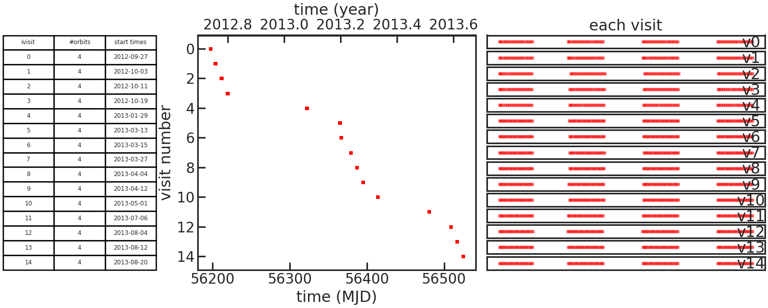
If the user didn’t set which_visits everything, two figures like this will be generated.
One with all visits and the other with only the ones set with which_visits.
Stage 02
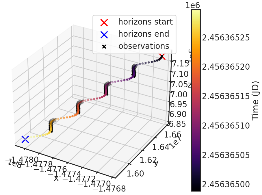
save_barycorr_plot/show_barycorr_plot
Example: True
Saves or shows a plot with the downloaded X,Y,Z positions of HST from the HORIZONS system by JPL during the observations.
Stage 03
Teff, logg, MH
Teff 3250logg 5.026MH 0.29effective Temperature (Teff), surface gravity (logg) and metallicity (MH) of the star.
Used to generate the stellar model. If the user only wants to use a blackbody spectrum, the code ignores logg and metallicity.
sm
Example: phoenix
The stellar model one wants to use. It will be then multiplied with the grism throughput (either G102 or G141) to create a reference spectrum for the wavelength calibration of the spectra.
Options:
k93models: THE 1993 KURUCZ STELLAR ATMOSPHERES ATLASck04models: THE STELLAR ATMOSPHERE MODELS BY CASTELLI AND KURUCZ 2004phoenix: THE PHOENIX MODELS BY FRANCE ALLARD AND COLLABORATORSblackbody: A blackbody spectrum using Planck’s lawThe stellar models (exluding the blackbody) are retrieved from https://archive.stsci.edu/hlsps/reference-atlases/cdbs/grid/
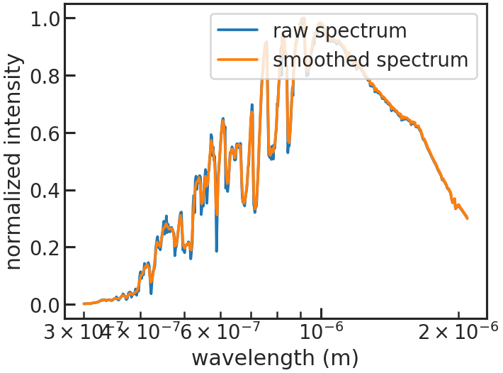
smooth/smooth_sigma
smooth Truesmooth_sigma 50If smooth is True, applies a Gaussian kernel smoothing to the stellar spectrum. This is recommended since the Kurucz and Phoenix stellar models have a higher resolution than the WFC3 grisms, which have native resolution of:
G141: 46.9 Angstrom/pixel dispersion
G102: 24.6 Angstrom/pixel dispersion
Gaussian smoothing the reference spectrum is discussed in detail in Deming et al. 2013. To follow their example and convolve the reference spectrum with a Gaussian with full-width at half maximum (FWHM) of 4 pixels, we use the relation FWHM = 2.35 * sigma. The value for the G141 grism is then 2.35 * 4 * 46.9 = 441
save_smooth_plot/show_smooth_plot
Example: True
Shows how the stellar spectrum was smoothed.
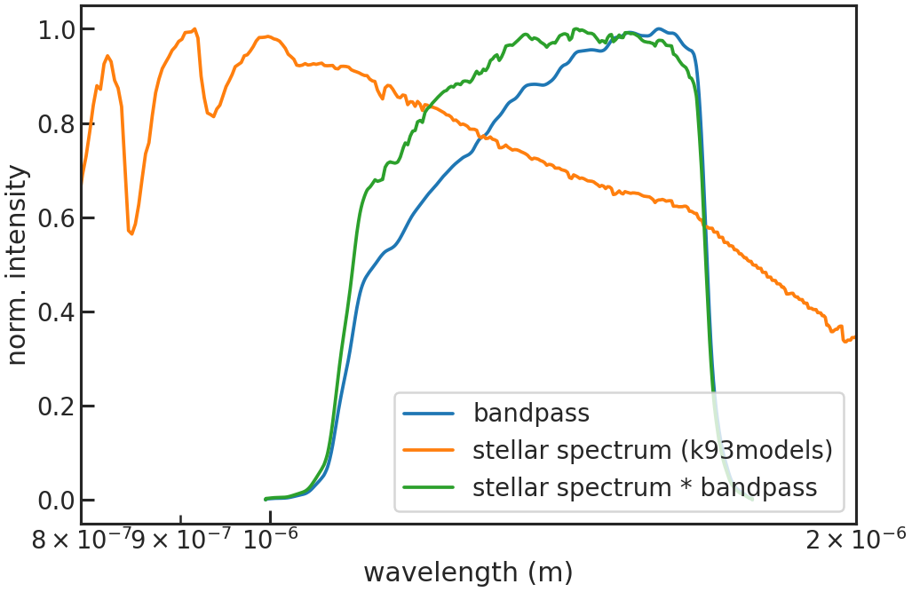
save_refspec_plot/show_refspec_plot
Example: True
Saves or shows a plot of the reference spectrum (stellar spectrum * bandpass).
Stage 10
di_rmin, di_rmax, di_cmin, di_cmax
di_rmin 120di_rmax 160di_cmin 5di_cmax 50These values specify a cutout around the target star. Below you will find an example:
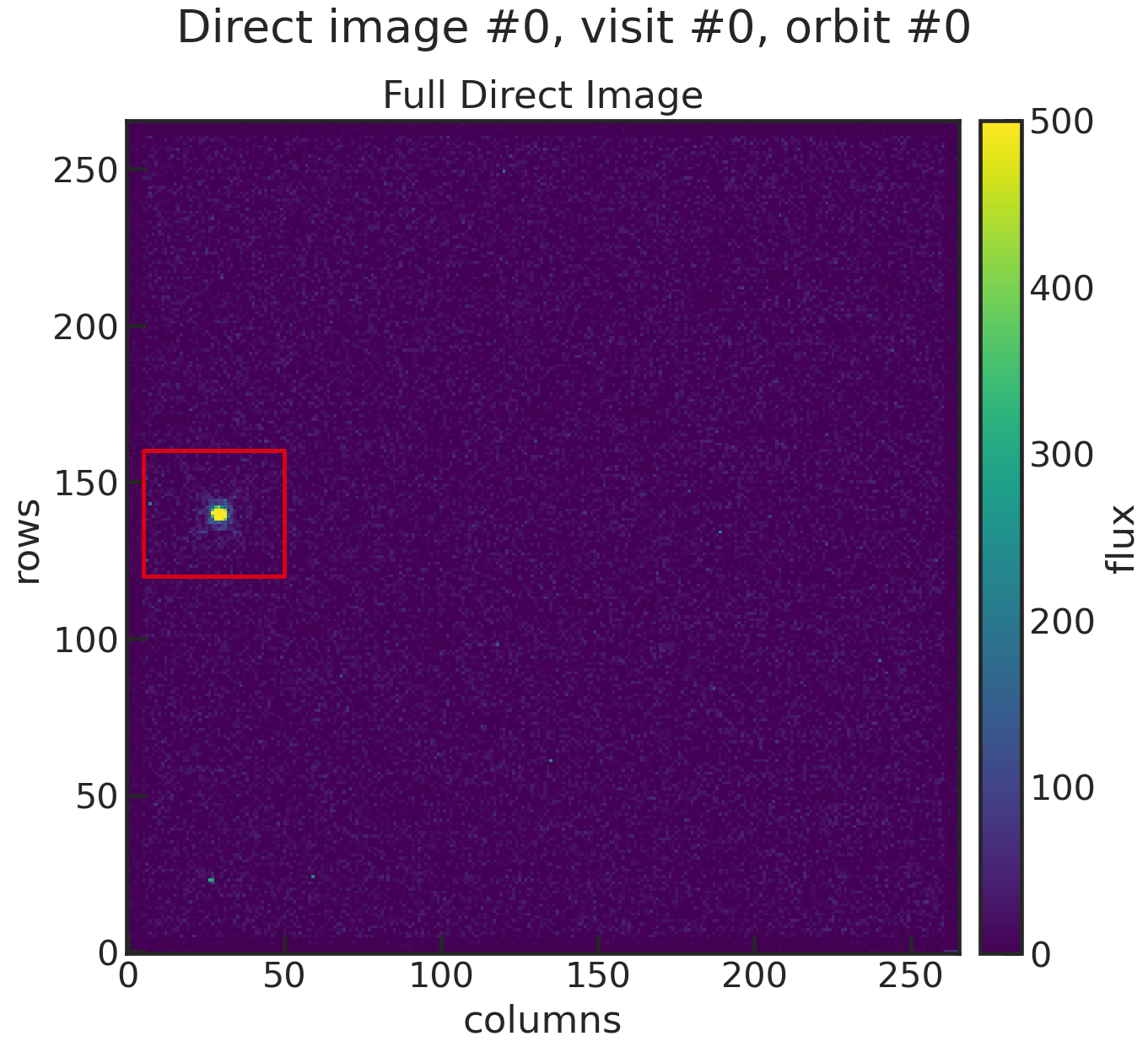
You can see that the cutout (red box in the plot) includes the star, so the centroid can be determined.
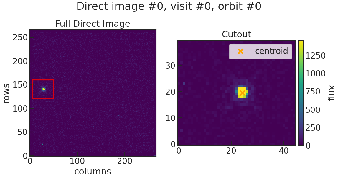
save_image_plot/show_image_plot
Example: True
Saves two plots for every direct image. The first one just shows the image with the location of the direct image cutout. The second plot shows the cutout on the left and the result of the 2D gaussian fit on the right. The gaussian fit only considers the cutout for the fit.
di_multi
di_multi mediandi_multi latestOptions: median or latest
Some observations have more than one direct image per orbit which were taken at the start of the orbit. In these cases the user can decide if they want to only use the most recent DI or a median of the DI positions in the orbit.
Stage 20
s20_testing/n_testing
s20_testing Truen_testing 1Runs s20 in testing mode. Only the first n_testing files will be analyzed then. E.g. if n_testing = 1, only the first file will be analyzed.
rmin/rmax
rmin 5rmax 261Can be set to remove rows from the top and bottom of the 2D array.
E.g. If the frame has the size of 266x266 and the user wants to cut off the
upper and lower 5 pixels they can use the same settings as in the example above.
Typically, for a 266x266 array, the user would set rmin 5 and rmax 261.
For 522x522 array, rmin 5 and rmax 517.
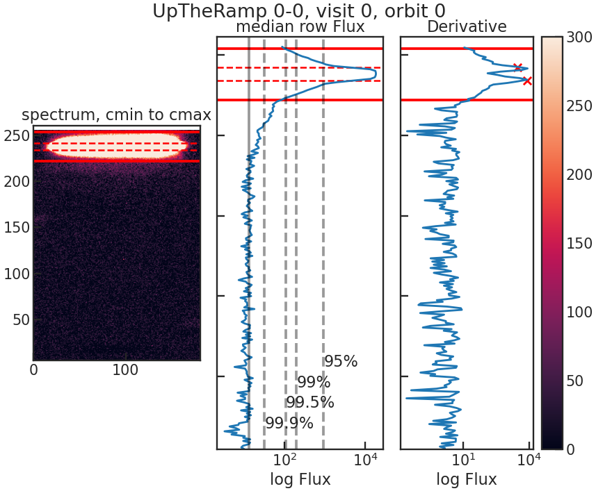
window
window 10Sets the size of the extraction window. PACMAN adaptively determines the best aperture in two steps:
identify the rows with the largest gradient in count rate
add
windowadditional rows above and below the rows identified in step 1
For example, if the biggest flux gradient occurs in row 35 and 55, and the user sets window 10,
the extraction aperture will be between rows 25 and 65.
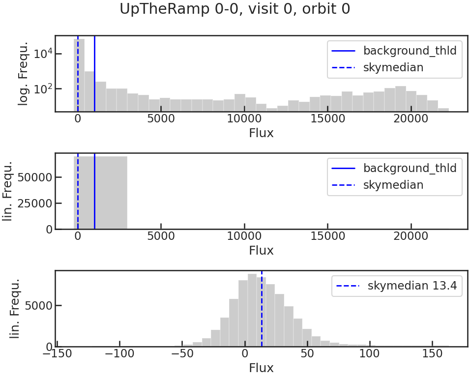
background_thld
background_thld 1000Sets a threshold for the background calculation. Pixels with a flux lower than background_thld electrons/second will be considered background. The background flux is then determined by taking the median flux of the pixels below this threshold.
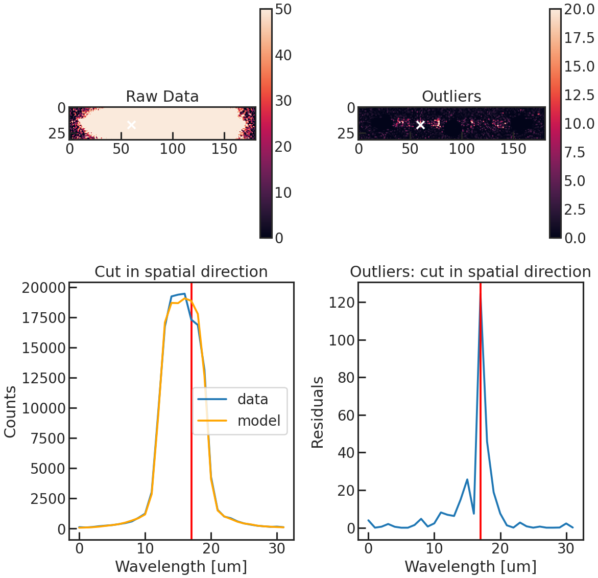
opt_extract
opt_extract TrueExtracts the spectrum using the optimal extraction routine from Horne et al. 1986.
If set to false, PACMAN performs a quick box extraction (simply adding up all the counts in the aperture). This gives a quick look at the spectra, but the following stages will break if opt_extract is false.
sig_cut, nsmooth
sig_cut 15nsmooth 9sig_cut: Specifies the outlier threshold for the optimal extraction. Outliers greater than sig_cut are masked.
If you have a lot of nans in your light curve you might want to increase the sig_cut value.
smooth: Number of pixels used for median-smoothing to create the spatial profile.
save_optextr_plot
Save plot showing some diagnostics from the optimal extraction.
correct_wave_shift
correct_wave_shift TrueInterpolates each spectrum to the wavelength scale of the reference spectrum, to account for spectral drift over the observation.
correct_wave_shift_refspec
uses the created reference spectrum during stage 03 for the wavelength calibration.
output
output TrueSaves the flux as a function of time and wavelength.
background_box & bg_rmin etc.
Do you want to calculate the median flux in a box to use as an estimate of the background flux?
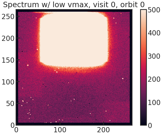
background_box Falsebg_rmin 100bg_rmax 400bg_cmin 40bg_cmax 100save_sp2d_plot/show_sp2d_plot
2D spectrum of the target with a low vmax value to see the background better.
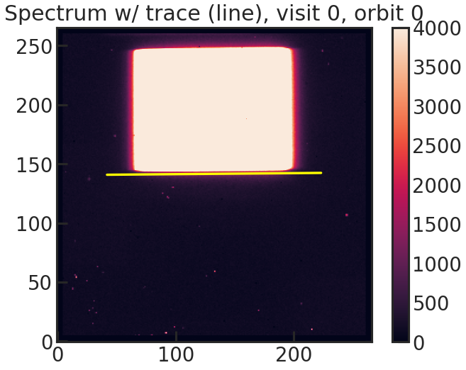
save_trace_plot/show_trace_plot
2D spectrum with the expected position of the trace based on the direct image.
save_bkg_hist_plot/show_bkg_hist_plot
Shows a histogram of the flux based on the difference of two consecutive up-the-ramp samples. This is why the user might see also negative fluxes.
save_utr_plot/show_utr_plot
Shows an up-the-ramp sample with the determined highest flux changes between two rows.
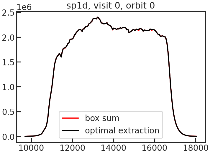
save_sp1d_plot/show_sp1d_plot
The 1D spectrum. The optimal extraction is shown in black, and the box extraction is shown in red.
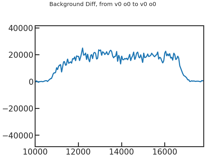
save_bkg_evo_plot/show_bkg_evo_plot
The determined background flux versus time.
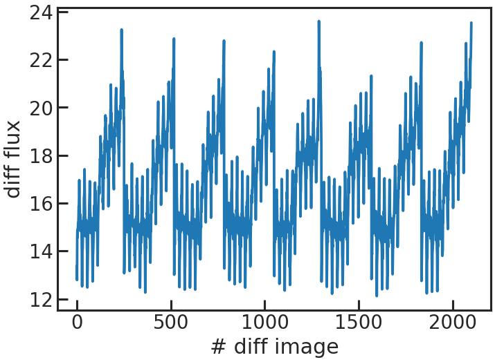
save_sp1d_diff_plot/show_sp1d_diff_plot
The difference between two consecutive 1D spectra.
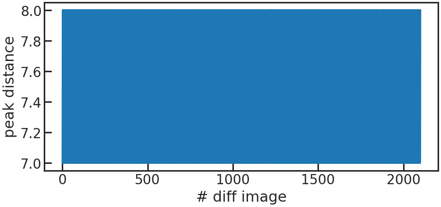
save_utr_aper_evo_plot/show_utr_aper_evo_plot
The determined aperture size over time. In this case the rows with the highest change in flux were either 7 or 8 pixels apart.
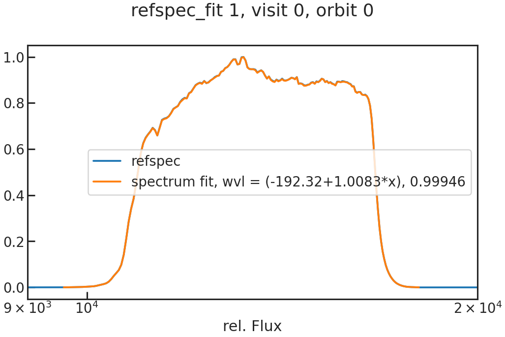
save_refspec_fit_plot/show_refspec_fit_plot
The fit of the 1D spectrum compared to the reference spectrum. In the first exposure in a visit, this reference spectrum is the product of the stellar spectrum with the grism throughput.
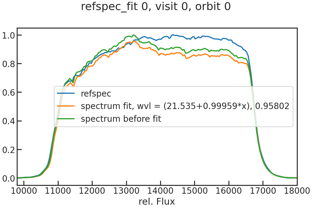
In the other exposures, the reference spectrum is the wavelength-calibrated first exposure in a visit.
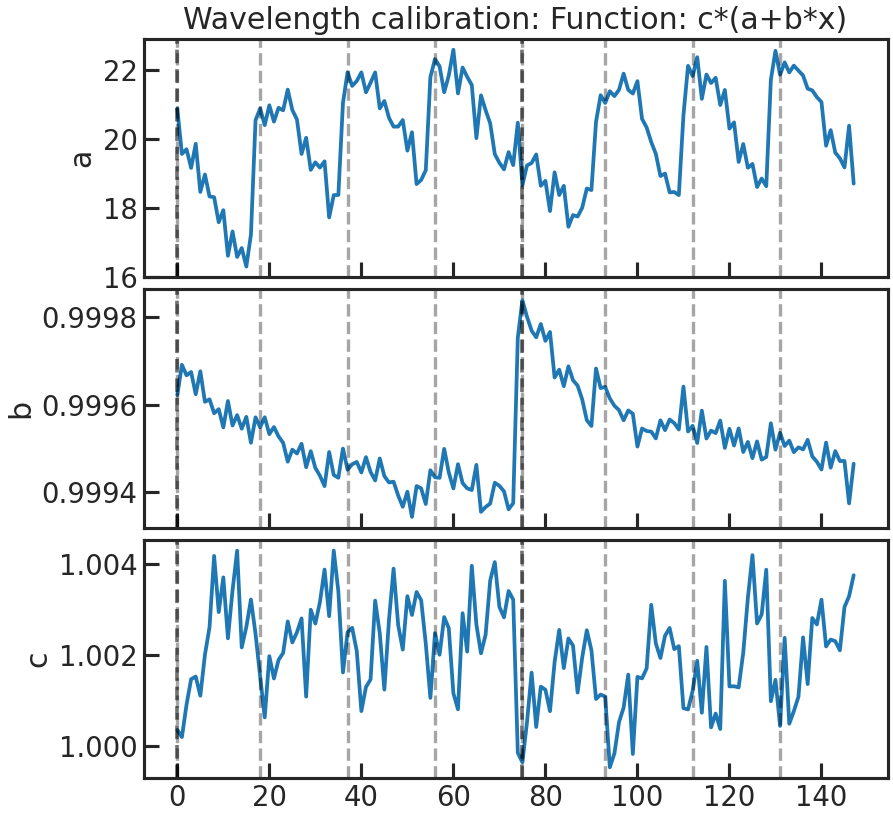
save_drift_plot/show_drift_plot
The fitted wavelength calibration parameters over time. We do a linear fit (a + b * wavelength) to the reference spectrum (which can be either a stellar model * instrument throughput or the first exposure in a visit depending on what the user chose in correct_wave_shift_refspec) and fit for the height. If a reference spectrum was a stellar model * the throughput, the first fit parameters of the fit of the 1d to the sm*throughput wont be shown in that plot.
First panel: a Second panel: b Third panel: height
Stage 21
s21_most_recent_s20/s21_spec_dir_path_s20
s21_most_recent_s20 Trues21_spec_dir_path_s20 NoneIf s21_most_recent_s20 is True, PACMAN automatically uses the most recent stage20 run directory.
If s21_most_recent_s20 is set to False, the user can set a path with the extracted data after s20:
s21_spec_dir_path_s20 /home/zieba/Desktop/Projects/Observations/Hubble/GJ1214_13021/stage20/s20_run_2022-02-11_17-44-56/wvl_min/wvl_max/wvl_bins
wvl_min 1.125wvl_max 1.65wvl_bins 12Start and end wavelengths for the spectroscopic light curves (microns). The wvl_bins parameter sets the number of wavelength channels.
use_wvl_list/wvl_edge_list
use_wvl_list Truewvl_edge_list [1.1,1.3,1.5,1.7]If the user wants to use a custom wavelength list for the binning, set use_wvl_list to True.
The units here are always microns.
There are two formats for a custom wvl_edge_list:
If entering a 1D array like wvl_edge_list [1.1,1.3,1.5,1.7], PACMAN will always create NON-OVERLAPPING bins. In this example, you would get 3 bins covering the following ranges: 1.1-1.3, 1.3-1.5, 1.5-1.7.
If entering a 2D array like wvl_edge_list [[1.0579,1.0677],[1.0604,1.0701],[1.0628,1.0726]], you will get the following three bins: 1.0579-1.0677, 1.0604-1.0701, 1.0628-1.0726.
This might be useful if you want to create OVERLAPPING bins. An example for that is searching for Helium with the G102 grism around 1083 nm, like in Spake et al., 2018.
Make sure you do not use spaces in any of these lists, otherwise it’s not readable to the code.
Stage 30
s30_myfuncs
Choose the functions to fit the data. The available functions are listed in models.
s30_fit_white
Fit the white light curve created in stage 20.
s30_fit_spec
Fit the spectroscopic light curves created in stage 21.
remove_first_exp
Removes the first exposure from every orbit.
remove_first_orb
Removes the first orbit from every visit.
remove_which_orb
Which orbits do you want to remove? E.g., if only the first choose [0]. If the first two, use [0,1].
rescale_uncert
Rescales the uncertainties for the sampler (MCMC or nested sampling), so that the reduced chi2red = 1. Note: This only happens if chi2red < 1 after least squared fit.
An alternative is to use uncmulti as a model in your fit. This will rescale the errorbars at every step of the sampler. The uncmulti value which the user will get after the sampling should be approximately the square root of the reduced chi square of the fit (i.e., uncmulti ~ sqrt(chi2_red)).
rescale_uncert_smaller_1
If this is True, PACMAN will also rescale the errorbars if chi2_red < 1, so that chi2_red = 1. This parameter was motivated by Colón+2020 (https://arxiv.org/abs/2005.05153): “For light curves where the best fit had a reduced chi-squared (chi2_red) greater than unity, we rescaled the per point uncertainties to achieve chi2_red = 1 before we ran the MCMC.”
So if one wants the same setup as mentioned in Colon+2020, one has to set rescale_uncert to True and rescale_uncert_smaller_1 to False.
run_clipiters
NOT TESTED
run_clipsigma
NOT TESTED
white_sys_path
Location of the white_systematics.txt file. Only needed if the user wants to use ‘divide_white’ as a model.
ld_model
ld_model 1Options:
1 = “linear” limb darkening
2 = “quadratic” limb darkening
kipping2013 = quadratic limb darkening in the Kipping2013 parameterization.
fix_ld
If true, PACMAN will use ExoTiC-LD to calculate limb darkening parameters and fix them during the fits.
ld_file
NOT TESTED but should give the possibility to use your own limb darkening file.
toffset
Subtracts an offset from the time stamps so that there is no problem with floating precision due to the size of dates in BJD.
run_verbose
If set to True, additional information is being outputted when running.
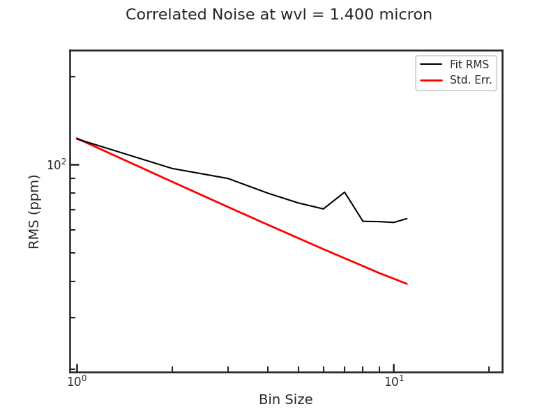
save_time_averaging_plot
The time averaging plot (formally known as Allan deviation plot). View this manuscript for more details: `Exoplaneteers Keep Calling Plots Allan Variance Plots When They Aren't <https://ui.adsabs.harvard.edu/abs/2025arXiv250413238K/abstract`_.
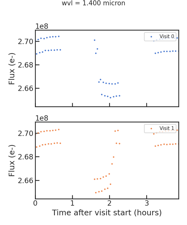
save_raw_lc_plot
Raw light curve plot
save_fit_lc_plot
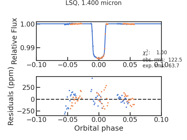
Plots the light curve fit without the instrumental systematics and only the astrophysical signal.
run_lsq
Runs the least square routine. Has to be True currently.
run_mcmc
Runs an MCMC using the emcee package.
run_nested
Runs nested sampling using the dynesty package.
ncpu
Number of cores used by emcee or dynesty. Use ncpu = 1, if you don’t want to use parallelization.
run_nsteps/run_nwalkers/run_nburn
Parameters for emcee.
nwalkers is explained here in the emcee API and run_nsteps here.
run_dlogz/run_nlive etc
run_dlogz 0.01run_nlive 400run_dynamic Falserun_dlogz_init 0.01run_nlive_init 80run_nlive_batch 100run_maxbatch 20run_bound multirun_sample autoParameters for dynesty.
If run_dynamic = False, then dynesty’s static mode will be used. The dynamic parameters (run_dlogz_init, run_nlive_init, run_nlive_batch, run_maxbatch, run_bound, run_sample) are well-explained in the dynesty API and in this tutorial The static parameters (run_dlogz, run_nlive, run_bound, run_sample) are expained in the dynesty API too.
The bound and sample parameters which are used by both the static and the dynamic mode are explained here.
lc_type
Currently not used.